Using the Plug-in
In the following I am going to demonstrate two examples of combining images in which I use the image registration plug-in in a preparatory step to align the images. In the first example I will show how to create an HDR image out of three exposure bracketed images. The images are slightly out of alignment as I took them without tripod. The second example is about a white stripe which my old scanner puts into the output images. I will show how to eliminate this stripe by combining two scans of the same object.
Common to both examples is the fact that the images cannot be aligned by simply moving the images in some direction. What we need in most cases is a combination of translation and rotation, and in some rare cases even scaling and shearing. This is where the plug-in comes handy and helps us fine-align the images before we go for the actual process of combining the images.
The images used in these examples can be downloaded from the project download page under the following link: https://sourceforge.net/projects/gimp-image-reg/files/examples/.
Example 1: Creating an HDR image
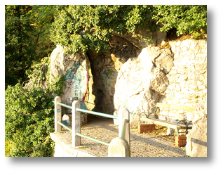
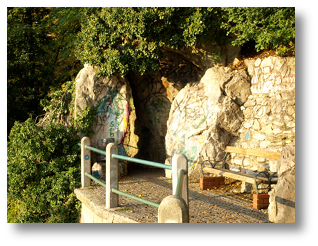
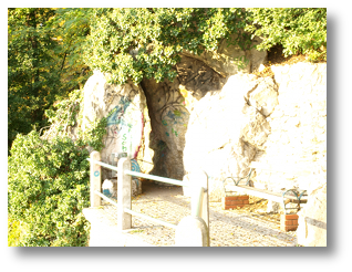
The photos serving as raw material for this example were taken on a sunny October afternoon at Schlossberg in Graz, Austria, as a series of exposure bracketed images with exposure values 0.0, -1.0, and +1.0:
 |
 |
 |
sb-1.jpg F-Number: f/16.0 Exposure time: 1/6 sec Exposure bias value: 0 EV |
sb-2.jpg F-Number: f/16.0 Exposure time: 1/13 sec Exposure bias value: -1 EV |
sb-3.jpg F-Number: f/16.0 Exposure time: 1/3 sec Exposure bias value: +1 EV |
The steps for creating a contrast enhanced image out of these photos will be the following:
- Load the images as layers into Gimp
- Align the images to minimize the displacements
- Combine the images using layer masks
Loading the images
Go to File
menu and Open as Layers
the images
sb-1.jpg,
sb-2.jpg, and
sb-3.jpg.
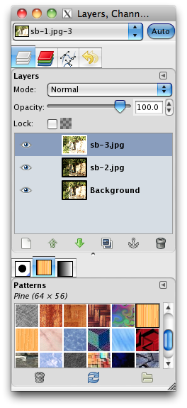
The just loaded images will appear as separate layers in the layer
panel. Gimp uses the name Background
for the first image, which
is sb-1.jpg in our case. Other layers have the same
name as the corresponding files.
Aligning the images
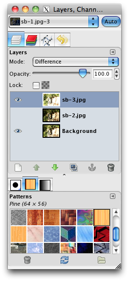
sb-2and set the layer mode of
sb-3to Difference.
We choose sb-1
(Background) as our reference image
and align sb-2
and sb-3
by applying the image
registration plug-in separately to each of them.
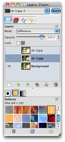
Let's start with sb-3
. First, we make sb-2
invisible
(by clicking off the eye symbol to the left of layer's icon)
and set the layer mode of sb-3
to Difference.
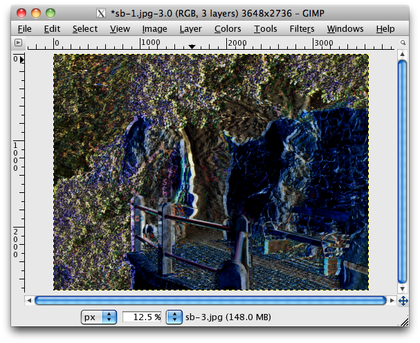
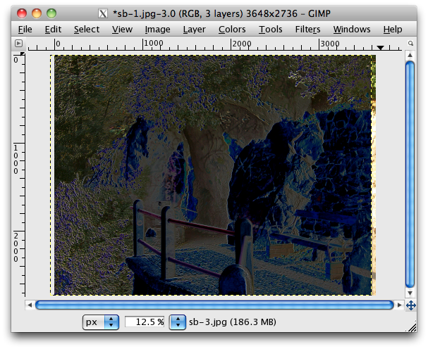
What we see now in Gimp's drawing area is the difference of
sb-3
to our reference image Background
. The difference
image is quite helpful in dealing with slightly displaced images, as
the bright edges give very useful clues to how much the images are
actually displaced.
As an optional intermediate step, we manually move sb-3
and
reduce its displacement relative to the reference image. It is not
necessary to achieve an exact match as we are going to apply the
registration plug-in anyway. However, by manually adjusting the layer
position we create a better starting point for the plug-in and thereby
reduce the number of necessary iterations.
For moving sb-3
, make sure that the corresponding layer is
selected (white frame in the layer panel), select Move
from the
Tools panel, click into the drawing area, and move the cursor while
keeping the mouse button pressed. You will see the bright areas in the
difference image changing in size. Try to make them as small and as
narrow as possible. Don't worry if you can't make them totally
disappear. The remaining differences will be taken care of by the
registration plug-in, which we are going to apply next.
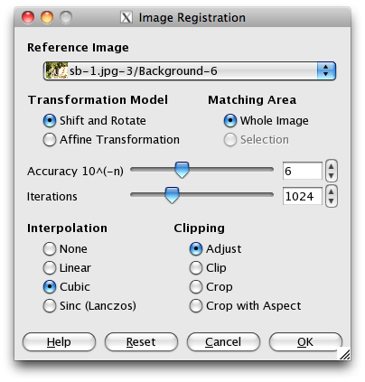
Reference Imagedenotes the layer against which we align the selected layer.
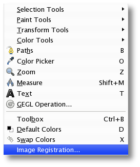
Now make sure that sb-3
is still selected, and choose
from Tools
menu the Image Registration
plug-in, which
you find as the last item in this menu.
This will pop up a dialog for setting the parameters and starting
the image registration. The reference image in this dialog denotes
the layer against which you wish to align the selected layer. We
select Background
as reference image and start the image
registration process by clicking OK.
sb-3to
Backgroundafter running the plug-in.
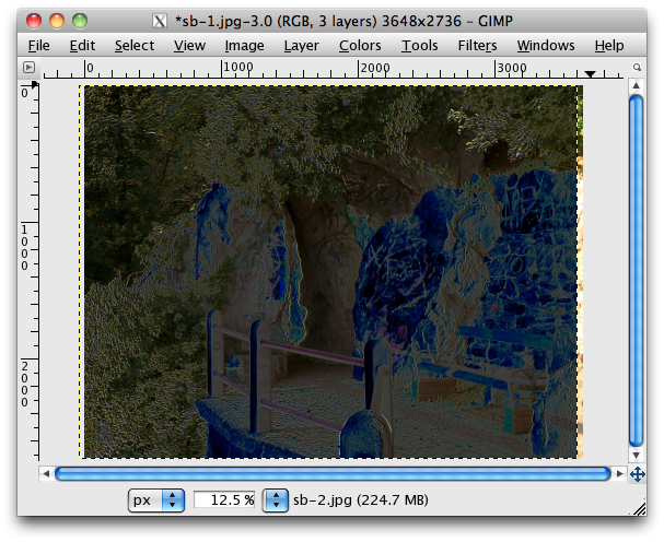
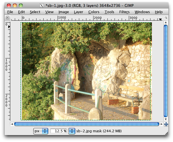
After a certain number of iterations, the plug-in will transform
sb-3
to minimize the remaining displacements with respect to
the reference image. The final result is shown in this screen
shot:
sb-3, select
sb-2, and set its mode to Difference.
Having finished the transformation step for sb-3
, we repeat
now the same procedure for sb-2
:
First we make sb-3
invisible and select sb-2
as the
layer we are going to operate on (note the white frame), and set its
mode to Difference to help see the existing
displacements.
sb-2after running the plug-in.
Afterwards, we manually reduce the displacements by moving the selected layer (optional) and apply the plug-in. The screen shot shows the difference image after running the plug-in.
Having aligned the images, we switch now both layers sb-2
and sb-3
back to Normal mode and go for combining
their intensities.
Combining the images
As the last step, we combine the layers by attaching a layer mask
to each of sb-2
and sb-3
. A layer mask is a gray-scale
image determining the transparency of the image, with white making
the corresponding pixels in the image fully opaque, and black making
them fully transparent. Values in between produce an effect of
partial transparency.
What we aim to achieve in this example is to enhance the dynamic range of the background image (EV=0) by taking
- dark areas from the overexposed image (sb-3), and
- bright areas from the underexposed image (sb-2).
We produce this effect by adding
- an inverted gray scale copy as layer mask to
sb-3
, and - a simple, i.e. non-inverted gray scale copy as layer mask to
sb-2
.
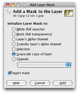
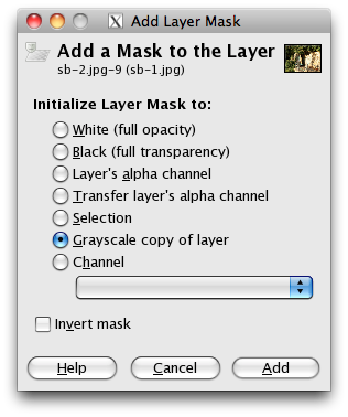
Note the inversion of the mask for the overexposed image.
For doing so, go to layer panel, right-click on the layer, and
select Add Layer Mask…
in the context menu. The corresponding
dialogs are shown in these screen shots.
This is the result of combining the exposure bracketed images.
You can achieve different results by deactivating any of
sb-2
or sb-3
, or by moving sb-2
up to make it the
top layer.
Example 2: Removing the White Stripe
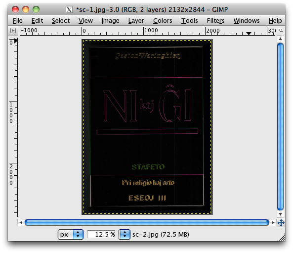
 |
 |
| sc-1.jpg | sc-2.jpg |
Ni kaj Ĝicover page taken on different positions on scan area.
In this example I am going to show how I combine two scans of the same object to remove the white stripe which my old scanner puts into the output images. The scans I am combining in this procedure are taken by placing the object on different positions on the scan area. By doing so I achieve that the annoying white stripe appears on different positions in the output images, so that I can take one of the images as background and cover the white stripe in it with a narrow rectangle of the second image in the same position.
As in the previous example, the steps for combining the scans into a
stripe free
image will be the following:
- Load the images as layers
- Align the images
- Combine the images to remove the stripe
Loading the images
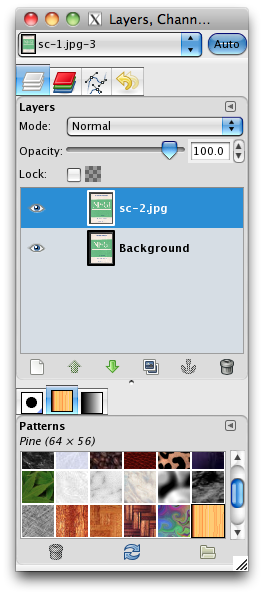
Go to File
menu and load the images
sc-1.jpg and sc-2.jpg as layers into
Gimp. The loaded images will appear as Background
and
sc-2.jpg
in the layer panel.
sc-2to difference to see its displacement relative to
Background.
After loading the images, set the mode of sc-2
to
difference to see its displacement relative to
Background
.
Aligning the images
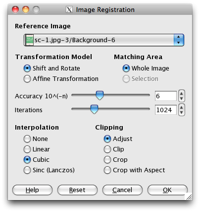
Make sure that sc-2
is selected (white frame in the layer
panel) and start the image registration plug-in from the Tools
menu. Accept the values presented in this dialog and run the plug-in
by pressing OK.
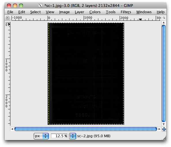
After a few iterations the plug-in will calculate the warp
parameters and transform the selected layer sc-2
to a perfect
match with the reference image Background
, indicated by an
almost black difference image as shown in this figure.
Combining the images
Having aligned the images, we now proceed to combine the images to
create one without a stripe. For doing so we take sc-1
as
background and make every part of sc-2
transparent, except a
narrow area around sc-1's white stripe, which we set opaque to make it
cover the underlying stripe in sc-1
. The following is a
detailed description of these steps.
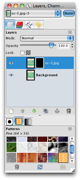
Reset sc-2's mode back to normal and attach a black, i.e. fully
transparent layer mask to it. The black layer mask will cause
sc-2
to disappear, and what we see now is the
Background
. Note the white frame around sc-2's layer mask,
indicating that the layer mask is selected for editing.
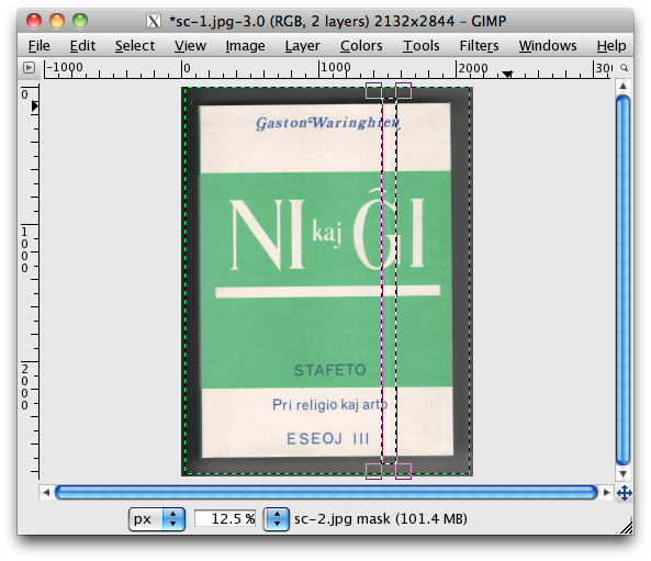
Choose the Rectangle Select Tool
from the Tools
panel
(e.g. by pressing R in the drawing area) and select a rectangular
area around sc-1's white stripe. This is going to be the area in sc-2,
which will cover sc-1.
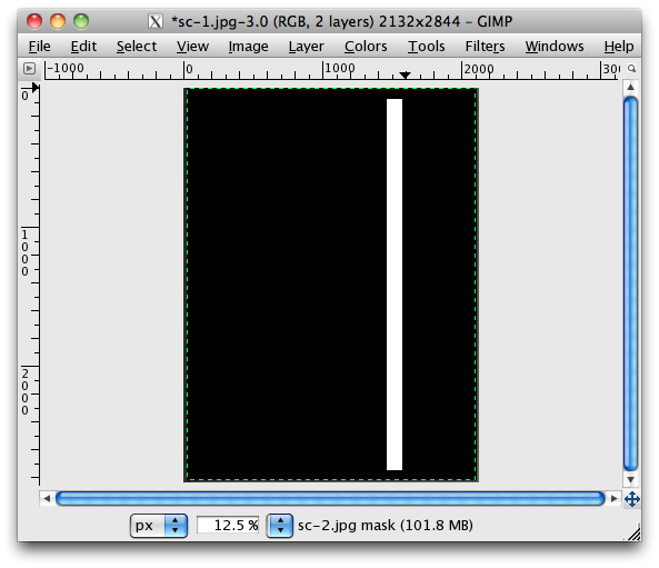
Show sc-2's layer mask and make sure it is still selected for
editing (white frame around the corresponding layer icon). Choose the
Bucket Fill Tool
from the Tools panel (e.g. by pressing Shift+B
in the drawing area) and fill the selected area with white.
The white rectangle in sc-2's layer mask corresponds to opaque area in sc-2, which now covers the white stripe in the underlying sc-1.
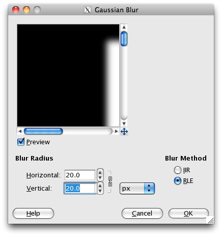
To soften the edges between sc-1 and sc-2, we apply a Gaussian blur to the white rectangle in sc-2's layer mask. Make sure to unselect everything or to select an area slightly larger than the white rectangle before applying the Gauss filter, otherwise the Gauss filter will be useless as its effect is limited to the selected area, which would be in our case only the white rectangle without the enclosing neighborhood.

The final result of combining the scans is shown in this figure. For making this image, I have slightly rotated the combined image and trimmed the dark borders contained in the original scans.